What is Subgraph Counting?
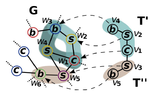
Subgraph counting goes under many names such as template matching or motif counting, but they all generally refer to counting the amount of a template T, that are present in a graph G. Refering to our illustration above, we may imagine that the template T (Here T is split on T’ and T”) on the right could fit in graph G in a few ways right? Well we would like to quantify just how many times T can fit in G. Such general problem manifests itself in many domains such as genomics, design of electronic circuits, and social network analysis.
How do we solve this problem?
We use the Color-coding approximation formulated by (Alon et. al., 1995) which can be presented the following way:
1. Establish a group of k distinct colors, where k is the number of vertices in the template T
2. Randomly color each vertex of graph G with the k distinct colors
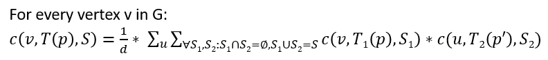
3. Count all colorful (meaning all vertices have a distinct color with no duplicates) copies of T in G rooted at every vertex v using
the following formula and diagram, where this is achieved by bottom-up dynamic programming. This means that we start by counting
the colorful copies of each one vertex tuple (this is trivial as they are all one distinct color), then we buid up to two vertex
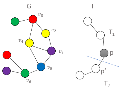
tuples and use the counts of the previous one-tuple step where we have the notion of an active child p, and a passive child p’.
Thus, we count all two-tuple embeddings where p is rooted at some vertex v in G, and p’ is its adjacent neighbor, then we multiply
their colorful combinations. We continue this process for 3-tuples by using the 2-tuple and 1-tuple counts, and finally we conclude
by finding the 5-tuple (final template count) by using the 3-tuple and 2-tuple counts. As a last counting step, we divide by d, where d is equal
to one plus the number of siblings of p’ which are roots of subtrees isomorphic to the subtemplate

 4. Sum up the template counts at all the vertices, then divide by q (which signifies the possibility of the template T being isomorphic to itself) as the following:
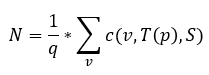 5. Multiply the final sum N by the probability of any given template T to be colorful as the following:
 6. If needed, repeat this process more times and average the count to obtain a more accurate measure (as this method yields an approximation)
Parallelizing the Color Coding algorithm via Harp Rotation:
In the initialization phase, each node in our distributed cluster will store a distinct part of the graph where we split the graph into p partitions, and we then use p nodes to do our computation.
Each node is then responsible for the chunk of vertices attributed to it, performing the count of the vertices contained in its own graph partition. You may imagine that depending on how the partitions are created,
the neighbors of certain vertices may be in other partitions, which makes it impossible for a node to locally do the count. This is where the rotation communication protocol comes in which is illustrated below.
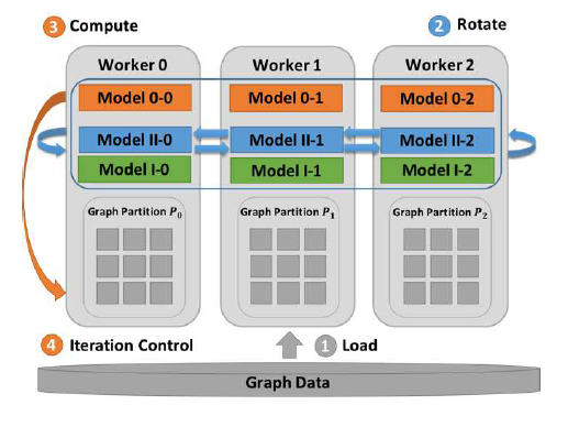 As seen from the illustration, we first load the data, then we compute the lowest level (single vertex of the template) of the dynamic programming color count which can be done on all of the partitions locally without the need for communication.
Then, we move up to the next level (two vertices with a direct child and a passive child) and compute the counts for the nodes that have local neighbors. However, the neighbors that are stored
on other partitions, must be rotated to that partition which have incident edges on those neighbors for the count to properly be computed. This repeats by rotating p times so that every partition
will have been exposed to all of the other partitions, hence being able to compute the Color Count at all of the vertices, considering all of the vertex neighbors. Finally, we continue this process, for the
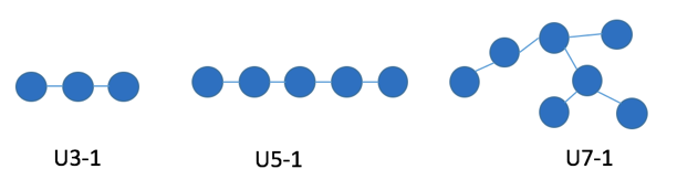
rest of the template substructures (i.e. 3 vertices, 5 vertices, etc… all depending on the template used), where a template of u5-1 (5 consecutive vertices connected by one edge forming a line) will
have a final template step of 5 vertices, by using the previous counts of 3 and 2. Where 3 is computed by 2 and 1, and 2 is computed by 1 and 1. This process is a bottom up dynamic programing scheme where
rotation and computation is alternated until all of the partitions have seen their vertex neighbors. Furthermore, this rotation/comptuation pattern happens for each dynamic programming step, starting with
the small sub-templates, and moving up to the final template at hand.
As seen from the illustration, we first load the data, then we compute the lowest level (single vertex of the template) of the dynamic programming color count which can be done on all of the partitions locally without the need for communication.
Then, we move up to the next level (two vertices with a direct child and a passive child) and compute the counts for the nodes that have local neighbors. However, the neighbors that are stored
on other partitions, must be rotated to that partition which have incident edges on those neighbors for the count to properly be computed. This repeats by rotating p times so that every partition
will have been exposed to all of the other partitions, hence being able to compute the Color Count at all of the vertices, considering all of the vertex neighbors. Finally, we continue this process, for the
rest of the template substructures (i.e. 3 vertices, 5 vertices, etc… all depending on the template used), where a template of u5-1 (5 consecutive vertices connected by one edge forming a line) will
have a final template step of 5 vertices, by using the previous counts of 3 and 2. Where 3 is computed by 2 and 1, and 2 is computed by 1 and 1. This process is a bottom up dynamic programing scheme where
rotation and computation is alternated until all of the partitions have seen their vertex neighbors. Furthermore, this rotation/comptuation pattern happens for each dynamic programming step, starting with
the small sub-templates, and moving up to the final template at hand.
Performance and Results
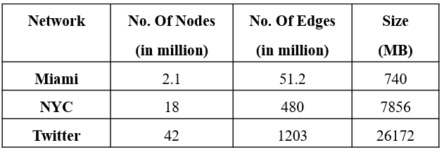
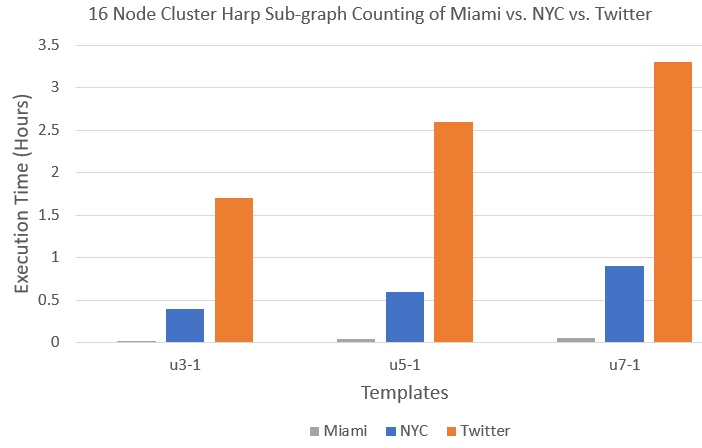
We set up a 16 node distributed Hadoop cluster on the Intel Haswell architecture where each node has 2 sockets, 12 cores per socket, and 2 threads per core, yielding 48 possible CPUs. Furthermore, each processor has the following model: Intel® Xeon® CPU E5-2670 v3 @ 2.30GHz. All the nodes have 128 GB memory and are connected by QDR InfiniBand. For our tests, JVM memory is set to “-Xmx73728m -Xms173728m”, and IPoIB is used for communication. Finally, we execute experiments on a 16 node cluster using 40 threads for each node, on templates 3-1, 5-1, and 7-1 (see Figure 1) for the following graphs (see Table 1) of which Miami and NYC have been generated via the (Chung and Lu, 2002) random graph generation process. In contrast, the Twitter dataset is a real dataset covering the follower network of 41 million users over a 7 month period in 2009.
Graphs
Templates Used
Results
Run Subgraph Counting Example
Data
You can download public data or download any graph data and turn it in the format below. Here are some datasets and templates for your reference.
Data Format
The format for the data should an adjacency list where each row is a sample vertex, followed by its neighbor vertices v1 v2,v6,v9,v12,. A practical example can be seen below where vertex 0
has 179-962 as its neighbors, and vertex 1 has 37-975 as its neighbors.
0	179,182,202,321,325,343,361,429,480,534,544,634,644,680,757,962,
1	37,71,201,341,354,369,416,426,439,459,509,510,597,624,719,813,823,858,901,975,
...
Usage
hadoop jar harp-java-0.1.0.jar edu.iu.sahad.rotation.SCMapCollective <number of map tasks> <useLocalMultiThread> <template> <graphDir> <outDir> <num threads per node>
Concrete Usage Example
hadoop jar harp-java-0.1.0.jar edu.iu.sahad.rotation.SCMapCollective 2 1 templates/u5-1.t ./inputgraphfileloc ./outputharpsahad 5
Assuming that you are using 2 compute nodes, have placed the template in the same location from which you are running this command, and have split the input file in half.
One way to split the file is by using the wc -l <inputfile> to get the total amount of lines where each line is a vertex. Then the split -l <total_amt_lines/2> which
will split this file into two files each having an equal amount of vertices. Note that if the files cannot be split evenly and the contents will overflow into a third file,
simply append the contents of this file to any of the other more “full” files using the linux cat file1 >> file2 command. Both of these files must then be placed in /inputgraphfileloc in HDFS. Finally,
here each node uses 5 threads and the output of the computation when it completes will be present at /outputharpsahad in HDFS.